
QFP-58: 5.8 GHz quad-feed, sequentially rotated CP patch (rev C)
Two-board air-dielectric patch antenna with four capacitively coupled probe feeds, driven 0/−90/−180/−270° by a two-stage Wilkinson network.
Rev B/C are retuned against openEMS (FDTD). Rev A's cavity-model sizing was wrong about the impedance level: the patch presents roughly 40-50 Ω per pin, not 100 Ω, and rev C additionally corrects the divider phase lengths. See "Simulation" below; src/qfp_sim.py reproduces every number.
The concept follows the Triple Feed Patch by Maarten Baert & Robin Theunis (CC BY-SA 4.0, maartenbaert.be). No TFP design files were used. All geometry is computed from a cavity model and microstrip synthesis (scikit-rf, Kirschning–Jansen).
Key parameters
| Item | Value |
|---|---|
| Centre frequency | 5.80 GHz (cavity model; bandwidth ≈10 % at VSWR 2) |
| Patch | Ø22.76 mm on the bottom side of the patch board (faces the ground) |
| Air gap | 4.00 mm copper-to-copper, target tolerance ±0.1 mm |
| Boards | both FR4 1.0 mm, 1 oz, 2 layers; feed Ø60 mm with an SMA flat, patch Ø23.96 mm |
| Feed pins | 4 × 1.0 mm Cu wire at r = 4.00 mm, drill 1.1 mm |
| Port impedance | ≈48 Ω active per pin (all four driven), at the end of the 2 mm matching section |
| Coupling disks | Ø3.6 mm on the patch-board top, ≈0.33 pF series, cancels ≈74–95 Ω of probe inductance |
| Patch antipad | Ø2.2 mm around a Ø1.4 mm ring (0.4 mm gap); feed-ground antipad Ø2.6 mm |
| Handedness | RHCP board as drawn; LHCP board is mirrored. The patch board is the same for both. |
Feed network (B.Cu of the feed board; F.Cu is a solid ground)
| Line | Z0 | Width | λg/4 |
|---|---|---|---|
| Input (SMA to stage-1 node) | 50 Ω | 1.883 mm | 7.03 mm |
| Stage-1 Wilkinson arms | 77.5 Ω | 0.794 mm | 7.31 mm |
| Branches to stage 2 | 60 Ω | 1.357 mm | 7.14 mm |
| Stage-2 Wilkinson arms | 77.5 Ω | 0.794 mm | 7.31 mm |
| Outputs | 50 Ω | 1.883 mm | 7.03 mm |
| Matching section at each pin | 100 Ω | 0.403 mm | 2.00 mm long (not λ/4) |
The 2 mm of thin 100 Ω line at each pin is a series-inductive matching element: it turns the patch's ≈41 − j30 Ω into ≈48 Ω, which is why the network runs at 50 Ω instead of rev A's 100 Ω.
The Wilkinson arms are lengthened by half the feeding stem width, measured from the stem edge.
Isolation resistors:
- R1 = 120 Ω (stage 1)
- R2, R3 = 100 Ω (stage 2)
- 0603, 1 %, thin film preferred
Path budget, SMA to pin (FR4 tan δ 0.02 → about 0.020 dB/mm, dominated by the dielectric):
| Pin | Angle | Phase | Length | Loss |
|---|---|---|---|---|
| P1 | 0° | 0° | 49.3 mm | 0.97 dB |
| P2 | 90° | −90° | 56.3 mm | 1.11 dB |
| P3 | 180° | −180° | 63.6 mm | 1.25 dB |
| P4 | 270° | −270° | 70.6 mm | 1.39 dB |
The power-averaged network loss is about 1.2 dB by hand, 1.31 dB in openEMS (which also includes radiation and the resistors).
Building
The only host requirement is Docker. ./run.sh builds the image on first use (about 15 minutes, since openEMS is compiled from source; 4.6 GB, 3.5 GB of which is the KiCad base image). Files are written as your user.
./run.sh                    # = --build: boards (RHCP feed in the root, the rest in kicad/), DRC, Gerbers, docs/
./run.sh --sim              # full antenna on the coarse mesh, ~4 min: quick check after a change
./run.sh --fullsim          # full antenna on the medium mesh, ~10 min: the reference numbers below
./run.sh --build --fullsim --cpus 5 --detach    # combine steps, limit cores, run in the background
./run.sh bash               # or any other command in the container
Simulation results land in sim_out/full_<hand><res><tag>/ (tag defaults to a timestamp), the log in sim_out/<tag>.log. The container is named qfp58-build (-2, -3, … for runs in parallel, or pick one with --name), so docker logs -f qfp58-build / docker stop qfp58-build find it. ./run.sh --help lists all options.
Files
QFP58-feed-RHCP.kicad_pro/.kicad_pcb   RHCP feed board, the showcase board in the root (the PCB-hosting
                                       repo renders a single root PCB); KiCad 10 project
QFP58-feed-RHCP-drc.rpt, fp-lib-table  its DRC report and footprint table
kicad/QFP58-feed-LHCP/                 LHCP feed board
kicad/QFP58-patch/                     patch board, Ø22.76 mm (the design value)
kicad/QFP58-patch-d23.06/, -d23.36/    spare patch boards, larger patch (see Fabrication)
kicad/QFP58.pretty/                    footprints (resistor, feed pin, SMA, M2 hole, coupling disk), shared
gerbers/*-fab.zip        Gerber X2 + separate PTH/NPTH Excellon, ready to upload
docs/svg/                per-layer SVG (B_Cu, F_Cu, Edge_Cuts), 1:1 mm, origin = antenna axis
docs/preview_*.png       layout previews
docs/design_report.json  every computed dimension, length, phase and loss
sim/                     openEMS results (plots, S-parameter CSVs, summaries)
src/                     generator and openEMS models
Dockerfile, run.sh       build container (KiCad 10, openEMS, locked Python deps); ./run.sh = full build
pyproject.toml, uv.lock  Python dependencies
KiCad notes
- Opening: open the
.kicad_prodirectly (KiCad 10 or newer). Each project has its ownfp-lib-table, all pointing at the onekicad/QFP58.pretty. - Network: drawn as real tracks and arcs on net
RF, so widths and lengths can be edited directly. - Ground:
GNDis a zone on F.Cu, drawn 0.25 mm inside the board edge like the simulated plane. Press B to refill after edits. - Patch: a zone on net
PATCH. It floats on purpose (it is capacitively coupled), so the project sets theisolated_coppercheck to ignore. - DRC: 0 violations on all boards (the patch's isolated copper is set to ignore, see above).
- SVG route instead: use File → Import → Graphics at scale 1:1. Copper comes in as graphic polygons with no net; convert them to zones or tracks if needed.
Fabrication
- Material: both boards must be 1.0 mm FR4 (εr ≈ 4.4), because the line widths depend on it. 1 oz copper, any finish, any mask colour.
- Soldermask: left on everything, including the patch. It shifts the patch by about −5 MHz and lowers line impedances slightly. This is not included in the synthesis.
- Patch variants: order the three patch boards together; they are small and all fit the same feed board.
The silkscreen shows the diameter. The simulated response centres slightly high, and FR4 from different fabs has shifted the TFP by about ±100 MHz, so the set brackets both:
| Board | Patch Ø | S11 dip | S11 < −20 dB | Gain 5.65 / 5.80 / 5.95 GHz | AR over beam, same |
|---|---|---|---|---|---|
QFP58-patch |
22.76 mm | 5.90 GHz | 5.54-6.30 GHz | 8.71 / 9.32 / 9.47 dBi | 1.90 / 1.14 / 1.40 dB |
QFP58-patch-d23.06 |
23.06 mm | 5.85 GHz | 5.51-6.23 GHz | 8.98 / 9.43 / 9.38 dBi | 1.62 / 1.04 / 1.64 dB |
QFP58-patch-d23.36 |
23.36 mm | 5.81 GHz | 5.48-6.18 GHz | 9.17 / 9.46 / 9.22 dBi | 1.39 / 1.06 / 1.91 dB |
openEMS full model, coarse mesh (gain within ~0.1 dB of the medium mesh, axial ratio only within ~0.4 dB), so read these as trends. Each 0.3 mm moves the response down roughly 40-70 MHz. 23.06 mm balances the two band edges best on the εr 4.4 the design assumes.
On JLC's laminate (Nan Ya NP-155F): the datasheet gives εr 4.2-4.4 and tan δ 0.014-0.016 at 1 GHz, a little lower again at 5.8 GHz. Simulated at εr 4.2 / tan δ 0.016, with the lines still drawn for 4.4 (the feed lines then run 1-2 Ω high and ~2 % short, which sequential rotation tolerates):
| Patch Ø | S11 < −20 dB | Gain 5.65 / 5.80 / 5.95 GHz | AR over beam, same |
|---|---|---|---|
| 22.76 mm | 5.61-6.32 GHz | 8.95 / 9.60 / 9.81 dBi | 2.21 / 1.28 / 1.19 dB |
| 23.06 mm | 5.58-6.25 GHz | 9.22 / 9.72 / 9.73 dBi | 1.90 / 1.08 / 1.41 dB |
| 23.36 mm | 5.56-6.19 GHz | 9.42 / 9.76 / 9.59 dBi | 1.62 / 0.98 / 1.65 dB |
The lower εr moves the response up by about one 0.3 mm step, and the lower loss adds ~0.3 dB of gain. On NP-155F, 23.36 mm is the balanced board and 23.06 mm the fallback if the real εr is nearer 4.4, so a two-board order should be 23.06 + 23.36 mm. Measure S11 and swap patch boards if the dip sits off 5.8 GHz.
BOM
| Ref | Part |
|---|---|
| R1 | 120 Ω 0603 1 % |
| R2, R3 | 100 Ω 0603 1 % |
| J1 | edge-launch SMA female for 1.0 mm PCBs |
| P1–P4 | 1.0 mm bare/tinned copper wire, about 8 mm each (not steel) |
| H1–H4 | M2 for mounting (optional, no RF effect) |
The J1 footprint is generic: signal pad 2.8 × 1.883 mm, ground pads 3.2 × 1.6 mm at ±2.9 mm, three vias per side, pads pulled back 0.25 mm from the edge. Check it against your connector's datasheet.
Assembly
- Feed-board parts: solder J1 and R1–R3 on the feed board's network side (B).
- Pins: push the four pins in from the ground side (F), solder them on the network side, and trim flush.
- Patch board: slide it over the pins with the coupling disks facing up and the patch copper facing down. Its rotation doesn't matter.
- Set the gap: hold 4.00 mm between the copper surfaces with a removable gauge, for example four 4 mm drill shanks. Check with calipers at four points.
- Finish: solder the pins to the disks, trim, and remove the gauge. Do not leave any dielectric spacer between the plates, because it pulls the frequency down.
Simulation (openEMS)
src/qfp_sim.py builds the FDTD models straight from the same geometry code, so any parameter change carries through. openEMS v0.0.36 and its Python bindings are built into the container, so every command runs via ./run.sh.
./run.sh python src/qfp_sim.py patch    --res fine              # patch + pins + disks, 4 ports, one excitation (4-fold symmetry)
./run.sh python src/qfp_sim.py network  --res medium            # feed board alone: SMA port + 4 ports at the interface
./run.sh python src/qfp_sim.py cascade                          # combine the two (no FDTD): S11, CP gain, axial ratio
./run.sh python src/qfp_sim.py full     --res medium            # whole antenna, single SMA port (slowest, the reference)
./run.sh python src/qfp_sim.py patch --res coarse --no-ff --set patch_d=25.0 rp=4.2   # fast tuning sweeps
Model settings: Gaussian excitation (5.8 GHz, fc 1.2 GHz), MUR boundaries ≥17 mm away, NF2FF box 4 cells inside, mesh ≤λ/20 in air and 0.10-0.13 mm on the lines, FR4 εr 4.4 with κ = 0.0284 S/m, stop at −40 dB energy. Copper is PEC (openEMS' conducting-sheet model went unstable on this mesh); add conductor loss by hand if needed. Isolation resistors are lumped elements across the pad gaps.
Results
Component models, rev B geometry (rev C only changed the divider phase lengths):
| Quantity | Value |
|---|---|
| Active match per pin (patch model, fine mesh) | ≤ −11 dB over 5.65-5.95 GHz, −10 dB from 5.50 to 6.00 GHz |
| Network input match / loss (medium mesh) | −22.8 dB at 5.8 GHz / 1.31 dB |
| Phases at the pins | 0 / −85 / 176 / 89° |
| S11 at the SMA (cascade) | ≤ −19 dB across 5.65-5.95 GHz |
| Half-power beamwidth | ≈52° |
Full model (whole antenna, single SMA port, medium mesh) - the reference result for rev C:
| Quantity | 5.65 GHz | 5.80 GHz | 5.95 GHz |
|---|---|---|---|
| RHCP realized gain, boresight | 8.74 dBi | 9.37 dBi | 9.55 dBi |
| Axial ratio, boresight | 2.11 dB | 0.94 dB | 0.70 dB |
| Axial ratio, mean over the beamwidth | 2.33 dB | 1.32 dB | 1.32 dB |
| Half-power beamwidth, narrowest-widest azimuth | 47-54° | 48-52° | 48-50° |
| Front-to-back (co-pol boresight vs strongest rear) | 13.7 dB | 13.3 dB | 12.1 dB |
| Radiated / incident power | 0.66 | 0.76 | 0.81 |
S11 at the SMA is better than -21.4 dB everywhere in 5.65-5.95 GHz (-29.5 dB at 5.8 GHz), below -20 dB from 5.62 to 6.32 GHz, and below -10 dB over the whole 5.0-6.6 GHz sweep, because the isolation resistors absorb what the patch reflects. (Numbers from the 2026-09-24 rerun in the build container; they reproduce the earlier run within 0.03 dB.)
Rev C differs from rev B only in phase_corr1 / phase_corr2: the lambda/4 differential arcs are stretched 7.4 % and the lambda/2 branch differential is shortened 2.8 %, calibrated against the openEMS network model. Phases at the pins are then 0 / -90.3 / -179.3 / -271.6 deg (rev B: 0 / -84.7 / -183.9 / -270.8).
What is left is amplitude, not phase: the pins receive -6.89 / -7.54 / -6.87 / -8.28 dB, i.e. the pair feeding one polarization is ~1.1 dB weak, which alone sets ~1 dB axial ratio. Within each divider the two outputs are a quarter wave apart, so they see the pin mismatch with opposite phase and the split becomes uneven; only a better patch match (now -11 to -15 dB) would improve it.
The axial ratio is still best above 5.8 GHz. Growing patch_d by ~0.3 mm moves the whole response down about 60 MHz and would balance 5.65 GHz against 5.95 GHz; that has not been simulated.
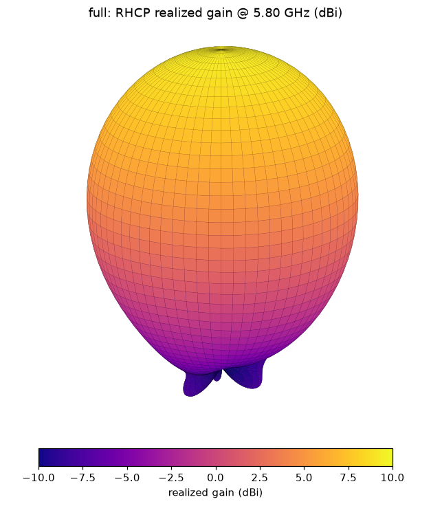
Radiation pattern (full model, medium mesh, 5.80 GHz)
| Simulated 3D radiation pattern | Simulated vertical cross-sections |
|---|---|
 |
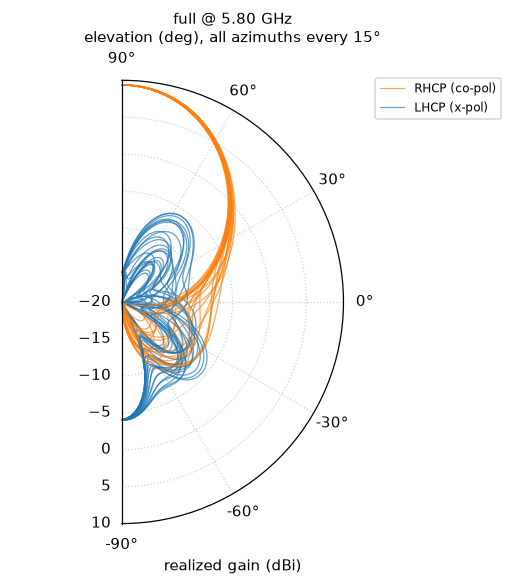 |
Left: RHCP realized gain; radius and colour are gain in dBi, clipped to −10…+10 dBi. Right: one curve per azimuth (every 15°), elevation +90° = boresight, −90° = straight back, co-pol RHCP and cross-pol LHCP. The spread of the orange curves is the beam's out-of-roundness; the blue ones show where the axial ratio degrades. The plots follow the layout of the TFP page, so the two can be compared directly. Band edges: sim/full/full_pattern3d_5.65GHz.png, ..._5.95GHz.png and the matching full_cuts_. Raw far-field data (θ step 2°, φ step 5°, RHCP/LHCP gain and axial ratio) is in sim/full/full_farfield_.npz.
Compared with the Triple Feed Patch
Same construction (two 1.0 mm FR4 boards, 4 mm air gap, probe feeds at 5.8 GHz); QFP-58 uses four feeds and Wilkinson dividers where the TFP uses three feeds and a branch-line-based hybrid. TFP figures are from maartenbaert.be (HFSS simulation, and anechoic-chamber / VNA measurement). QFP-58 figures are openEMS, full model, medium mesh; nothing here is measured.
| QFP-58 rev C (openEMS) | TFP (HFSS) | TFP (measured) | |
|---|---|---|---|
| Gain, boresight, 5.8 GHz | 9.37 dBi | 9.4 dBi | 9.3 dBi |
| Axial ratio, averaged over the beam | 1.32 dB | 1.06 dB | 1.21 dB |
| Efficiency | 0.76 radiated/incident | 81 % | 74 % |
| Half-power beamwidth | 48-52° | 55° | 55° |
| S11 < −20 dB | 5.62-6.32 GHz (700 MHz) | 5.47-6.13 GHz (660 MHz) | ~800 MHz |
On simulation the two are level: same gain, similar efficiency and bandwidth. The TFP's simulated axial ratio is ~0.25 dB better, and its beam is slightly wider. QFP-58's match stays below −10 dB over the whole 5.0-6.6 GHz sweep. Caveats: the efficiency definitions may differ (ours includes the feed network and mismatch, but not copper loss or the SMA), and the HFSS and openEMS models were set up independently. A measured comparison needs hardware.
Sensitivities and tuning
- Air gap: +0.1 mm gives roughly −25 to −50 MHz. The TFP author measured about −100 MHz from a 0.2 mm spacer error.
- FR4 εr: ±0.2 puts roughly ±3° of phase error on the λ/2 branch. Sequential rotation tolerates this well.
- Resistor power: R2 and R3 absorb the patch-port mismatch. At VSWR 2 on the pins, each takes about 5.5 % of the input power, so 0603 (0.1 W) is fine up to about 1 W.
- Model limits: the model is analytic. T-junctions, line-to-line coupling and connector transitions were not EM-simulated, so run openEMS or a VNA prototype before building a batch.
- Retuning: edit
Pinsrc/qfp_geom.pyand rerun./run.sh.